-
Course Information
Meet the Teaching Team -
Course Dataset 1
-
Course Dataset 2
-
MODULE A1: INTRODUCTION TO STATISTICS USING R, STATA, AND SPSSA1.1 What is Statistics?
-
A1.2.1a Introduction to Stata
-
A1.2.2b: Introduction to R
-
A1.2.2c: Introduction to SPSS
-
A1.3: Descriptive Statistics
-
A1.4: Estimates and Confidence Intervals
-
A1.5: Hypothesis Testing
-
A1.6: Transforming Variables
-
End of Module A11 Quiz
-
MODULE A2: POWER & SAMPLE SIZE CALCULATIONSA2.1 Key Concepts
-
A2.2 Power calculations for a difference in means
-
A2.3 Power Calculations for a difference in proportions
-
A2.4 Sample Size Calculation for RCTs
-
A2.5 Sample size calculations for cross-sectional studies (or surveys)
-
A2.6 Sample size calculations for case-control studies
-
End of Module A21 Quiz
-
MODULE B1: LINEAR REGRESSIONB1.1 Correlation and Scatterplots
-
B1.2 Differences Between Means (ANOVA 1)
-
B1.3 Univariable Linear Regression
-
B1.4 Multivariable Linear Regression
-
B1.5 Model Selection and F-Tests
-
B1.6 Regression Diagnostics
-
End of Module B11 Quiz
-
MODULE B2: MULTIPLE COMPARISONS & REPEATED MEASURESB2.1 ANOVA Revisited – Post-Hoc Testing
-
B2.2 Correcting For Multiple Comparisons
-
B2.3 Two-way ANOVA
-
B2.4 Repeated Measures and the Paired T-Test
-
B2.5 Repeated Measures ANOVA
-
End of Module B21 Quiz
-
MODULE B3: NON-PARAMETRIC MEASURESB3.1 The Parametric Assumptions
-
B3.2 Mann-Whitney U Test
-
B3.3 Kruskal-Wallis Test
-
B3.4 Wilcoxon Signed Rank Test
-
B3.5 Friedman Test
-
B3.6 Spearman’s Rank Order Correlation
-
End of Module B31 Quiz
-
MODULE C1: BINARY OUTCOME DATA & LOGISTIC REGRESSIONC1.1 Introduction to Prevalence, Risk, Odds and Rates
-
C1.2 The Chi-Square Test and the Test For Trend
-
C1.3 Univariable Logistic Regression
-
C1.4 Multivariable Logistic Regression
-
End of Module C11 Quiz
-
MODULE C2: SURVIVAL DATAC2.1 Introduction to Survival Data
-
C2.2 Kaplan-Meier Survival Function & the Log Rank Test
-
C2.3 Cox Proportional Hazards Regression
-
C2.4 Poisson Regression
-
End of Module C21 Quiz
-
A Note about the Fossa Certificate


Learning Outcomes
By the end of this section, students will be able to:
- Explore the data with correlations and scatterplots.
- Use an ANOVA to test for a difference in means across a categorical variable.
- Conduct univariable and multivariable linear regression
- Check the regression diagnostics of a linear model.
You can download a copy of the slides here: B1.6 Regression Diagnostics
Video B1.6 – Regression Diagnostics (9 minutes)
B1.6 PRACTICAL: Stata
One of the final steps of any linear regression is to check that the model assumptions are met. Satisfying these assumptions allows you to perform statistical hypothesis testing and generate reliable confidence intervals.
Here we are going to practice checking the normality and homoscedasticity of the residuals.
Checking Normality of Residuals
We need to make sure that our residuals are normally distributed with a mean of 0. This assumption may be checked by looking at a histogram or a Q-Q-Plot.
To look at our residuals, we use the post-estimation command ‘predict’ after the multivariable command we used above in B1.4a with bmi_grp4, ldlc and currsmoker.
predict sbp_r, resid
I have called my new variable “sbp_r”, and the option “resid” specifies that I want residuals rather than the default predicted linear values.
Then I can use the ‘sum’ command to check the mean, and then plot a histogram.
sum sbp_r
hist sbp_r
Checking Homoscedasticity
One of main assumptions of ordinary least squares linear regression is that there is homogeneity of variance (i.e. homoscedasticity) of the residuals. If the variance of our residuals is heteroscedastic then this indicates model misspecification. To check this we plot the values of our residuals against the fitted (predicted) values from our regression, and we hope to see a random scatterplot with no pattern. If we see a pattern, i.e. the scatterplot gets wider or narrower at a certain range of values, then this indicates heteroscedasticity and we need to re-evaluate our model.
Stata’s command for this is ‘rvfplot’. After you run your multivariable model, type:
rvfplot, yline(0)
Question B1.6: Examine your residuals from the multivariable regression in B1.4. Does this model appear to violate the assumptions of normality and homoscedasticity?
Answer
The mean of the residuals is 0, which is one assumption fulfilled.

The histogram of the residuals also appears normal:

When looking at the rvfplot, we see:

There appears to a be a random ball of dots, with no pattern. This is what we want. There does not appear to be heteroscedasticity.
B1.6 PRACTICAL: SPSS
One of the final steps of any linear regression is to check that the model assumptions are met. Satisfying these assumptions allows you to perform statistical hypothesis testing and generate reliable confidence intervals.
Here we are going to practice checking the normality and homoscedasticity of the residuals.
Checking Normality of Residuals
We need to make sure that our residuals are normally distributed with a mean of 0. This assumption may be checked by looking at a histogram or a Q-Q-Plot.
To do this in SPSS, we need to first save the residuals. When you are in the General Linear Model window click on the Save button on the right hand side. Then tick the box for Unstandardized Residuals. Press continue and run the test as normal.

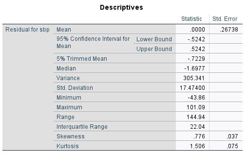
SPSS will output your residuals as a new variable. You can run descriptive statistics on this variable as outlined in Module A1.
Select
Analyze >> Descriptive >> Explore.
Select the option for Histogram within the Plots tab. You can deselect all other plot types so you don’t end up with too much output.
Checking Homoscedasticity
One of main assumptions of ordinary least squares linear regression is that there is homogeneity of variance (i.e. homoscedasticity) of the residuals. If the variance of our residuals is heteroscedastic then this indicates model misspecification. To check this we plot the values of our residuals against the fitted (predicted) values from our regression, and we hope to see a random scatterplot with no pattern. If we see a pattern, i.e. the scatterplot gets wider or narrower at a certain range of values, then this indicates heteroscedasticity and we need to re-evaluate our model.
To do this in SPSS you also need to save your unstandardized predicted values. Go back to your General Linear Model, open the Save tab again and select Unstandardized Predicted Values as well as Unstandardized Residuals.
Then create a scatter plot of these in the same way as you did in B1.1.
Examine your residuals from the multivariable regression in B1.4. Does this model seem to violate the assumptions of normality and homoscedasticity?
Answer
The mean of the residuals is 0, which is one assumption fulfilled.

The histogram of the residuals also appears normal.
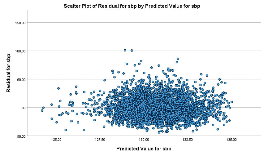
When looking at the scatter plot there appears to a be a random ball of dots, with no pattern. This is what we want. There does not appear to be heteroscedasticity.
B1.6 PRACTICAL: R
One of the final steps of any linear regression is to check that the model assumptions are met. Satisfying these assumptions allows you to perform statistical hypothesis testing and generate reliable confidence intervals.
Here we are going to practice checking the normality and homoscedasticity of the residuals.
Checking Normality of Residuals
We need to make sure that our residuals are normally distributed with a mean of 0. This assumption may be checked by looking at a histogram or a Q-Q-Plot.
To look at our residuals, we can use the function resid(). This function extracts the model residuals from the fitted model object (for example, in our case we would type resid(fit1)).
To check our residuals from the model we fit in B1.4 we would type:
hist(resid(fit5), main=”Histogram of the residuals”, xlab=”Residuals”)
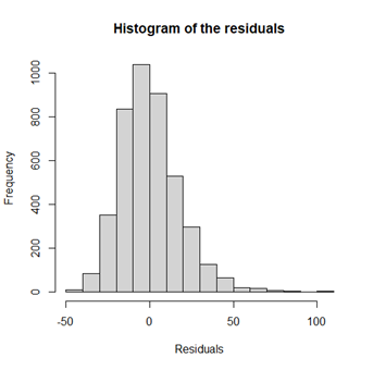
> sum(resid(fit5))
[1] 4.768824e-12
It appears that our residuals are normally distributed with zero mean.
Checking Homoscedasticity
One of main assumptions of ordinary least squares linear regression is that there is homogeneity of variance (i.e. homoscedasticity) of the residuals. If the variance of our residuals is heteroscedastic then this indicates model misspecification, similar to the reasons discussed before.
To check homogeneity in variance this we plot the values of the residuals against the fitted (predicted) values from the regression model. If the assumptions is satisfied we should see a random scatter of the points with no pattern. If we see a pattern, i.e. the scatterplot gets wider or narrower at a certain range of values, then this indicates heteroscedasticity and we need to re-evaluate our model. To plot the residuals versus the fitted values, we can use plot(resid(fit5) ~ fitted(fit5), …).
> plot(resid(fit5) ~ fitted(fit5), main=”The residuals versus the fitted values”, xlab=”Fitted values”, ylab=”Residuals”, cex=0.8)
> abline(0,0, col=2)
Question B1.6: Examine your residuals from the multivariable regression in B1.4. Does this model appear to violate the assumptions of homoscedasticity?
Answer

There appears to be a random ball of dots, with no pattern. This is what we want. There does not appear to be heteroscedasticity.