-
Course Information
Meet the Teaching Team -
Course Dataset 1
-
Course Dataset 2
-
MODULE A1: INTRODUCTION TO STATISTICS USING R, STATA, AND SPSSA1.1 What is Statistics?
-
A1.2.1a Introduction to Stata
-
A1.2.2b: Introduction to R
-
A1.2.2c: Introduction to SPSS
-
A1.3: Descriptive Statistics
-
A1.4: Estimates and Confidence Intervals
-
A1.5: Hypothesis Testing
-
A1.6: Transforming Variables
-
End of Module A11 Quiz
-
MODULE A2: POWER & SAMPLE SIZE CALCULATIONSA2.1 Key Concepts
-
A2.2 Power calculations for a difference in means
-
A2.3 Power Calculations for a difference in proportions
-
A2.4 Sample Size Calculation for RCTs
-
A2.5 Sample size calculations for cross-sectional studies (or surveys)
-
A2.6 Sample size calculations for case-control studies
-
End of Module A21 Quiz
-
MODULE B1: LINEAR REGRESSIONB1.1 Correlation and Scatterplots
-
B1.2 Differences Between Means (ANOVA 1)
-
B1.3 Univariable Linear Regression
-
B1.4 Multivariable Linear Regression
-
B1.5 Model Selection and F-Tests
-
B1.6 Regression Diagnostics
-
End of Module B11 Quiz
-
MODULE B2: MULTIPLE COMPARISONS & REPEATED MEASURESB2.1 ANOVA Revisited – Post-Hoc Testing
-
B2.2 Correcting For Multiple Comparisons
-
B2.3 Two-way ANOVA
-
B2.4 Repeated Measures and the Paired T-Test
-
B2.5 Repeated Measures ANOVA
-
End of Module B21 Quiz
-
MODULE B3: NON-PARAMETRIC MEASURESB3.1 The Parametric Assumptions
-
B3.2 Mann-Whitney U Test
-
B3.3 Kruskal-Wallis Test
-
B3.4 Wilcoxon Signed Rank Test
-
B3.5 Friedman Test
-
B3.6 Spearman’s Rank Order Correlation
-
End of Module B31 Quiz
-
MODULE C1: BINARY OUTCOME DATA & LOGISTIC REGRESSIONC1.1 Introduction to Prevalence, Risk, Odds and Rates
-
C1.2 The Chi-Square Test and the Test For Trend
-
C1.3 Univariable Logistic Regression
-
C1.4 Multivariable Logistic Regression
-
End of Module C11 Quiz
-
MODULE C2: SURVIVAL DATAC2.1 Introduction to Survival Data
-
C2.2 Kaplan-Meier Survival Function & the Log Rank Test
-
C2.3 Cox Proportional Hazards Regression
-
C2.4 Poisson Regression
-
End of Module C21 Quiz
-
A Note about the Fossa Certificate


Learning Outcomes
By the end of this section, students will be able to:
- Calculate and interpret a chi-squared test of association
- Calculate and interpret a chi-squared test for trend
You can download a copy of the slides here: Video C1.2a
Video C1.2a – The Chi-Square Test (7 minutes)
You can download a copy of the slides here: Video C1.2b
Video C1.2b – Test for Linear Trend (5 minutes)
C1.2 PRACTICAL: Stata
Performing the chi-square test for association
We want to look at the association of age group with fatal CVD. First produce a table using the ‘tab’ command:
tab age_grp cvd_death
In order to obtain estimates of CVD prevalence by age group and a chi-square test for association, we need to include row percentages in the table by typing the following:
tab age_grp cvd_death, row chi
The output should look like this:

Question C1.2a: Is there an association between age group and fatal CVD? Just looking at a cross-tabulation table without doing any additional steps, are you able to tell which age groups are different from each other?
Answer
The chi-square test statistic is shown below the table and is X2 = 221.7 on 3 df (chi2(3)) which gives a p-value of Pr = 0.000. When Stata says that the p-value equals 0.000 then this should be reported as p<0.001.
The p value of the chi-square test is highly significant (p<0.001), suggesting that we can reject the null hypothesis that there is no difference in true fata CVD prevalence across different age groups. While we can observe in the row percentages that fatal CVD prevalence is the highest at older ages, and lowest at younger ages, the chi-square test is a global test so it just tells us there is a difference somewhere in the table; it does not tell us which groups are different nor does it tell us about the nature of the association (e.g if it is positive or negative).
Performing the chi-square test for linear trend (Cochran-Armitage test)
The chi-square test for linear trend (also called the Cochran-Armitage test for linear trend) is obtained using the mhodds command. The setup of this command is:
mhodds var_case expvar [,options]
It is used with case-control and cross-sectional data, and it estimates the ratio of the odds of failure (i.e. disease) for two categories of expvar. It then tests whether this odds ratio is equal to 1. When expvar has more than two categories, use the option “compare(v_1, v_2)” to indicate the categories you want compared. If the “compare” option is not specified and there are more than 2 categories, then mhodds calculates an estimate of the odds ratio for a 1 unit increase in expvar.
To tell Stata that we want it to do the trend test, we do not specify the compare option:
mhodds cvd_death age_grp
The output should look like this:
Score test for trend of odds with age_grp
——————————————————————–
Odds ratio chi2(1) P>chi2 [95% conf. interval]
——————————————————————–
1.936917 216.11 0.0000 1.773504 2.115388
——————————————————————–
Note: The Odds ratio estimate is an approximation to the odds ratio
for a one-unit increase in age_grp.
Here, ‘chi2(1)’ refers to the chi-square test for linear trend, which yields a highly significant p-value. The resulting odds ratio represents the odds ratio for fatal CVD associated with any two adjacent groups of age group. In other words, the odds ratio for 71-75 versus 60-70 years of age is 1.94, as is the odds ratio for 76-80 versus 71-75, and the odds ratio for 81-95 versus 76-80.
Question C1.2b.i: Obtain the prevalence of prior diabetes in the different groups of BMI. What happens to diabetes prevalence as the BMI group increases?
Question C1.2b.ii: Perform a chi-square test of linear trend. What is the null hypothesis and what do the results of this test suggest?
C1.2b Answers
Answer C1.2b.i The prevalence of diabetes increases from 8% (underweight) to 5% (normal weight) to 8.8% in the group with obesity.

Answer C1.2b.ii The chi-square test for linear trend is obtained using the mhodds command. The chi-square value (for 1 degree of freedom) is 5.8 and the p-value=0.02. There is evidence of a significant linear trend, and we can reject the null hypothesis that there is no association between diabetes status and BMI group.
C1.2 PRACTICAL: SPSS
Chi-squared test of association
We want to look at the association between age group and fatal CVD. This test does not require calculation of risk ratios, so it does not matter how the binary variables are coded in SPSS. In these examples we have used the default of No= 0 and Yes =1.
We will first run the Chi squared test of association.
Select
Analyze >> Descriptives >> Crosstabs
Add age_grp and cvd_death variables to the rows and columns boxes as in the last practical. Click on ‘Cells’ and make sure you are showing observed counts and at least row level percentage values. Then click on ‘Statistics’ and tick the box next to ‘Chi-square’. Press ‘Continue’ and the then ‘OK’ to run the test.

Question C1.2a: Is there an association between age group and fatal CVD? Just looking at a cross-tabulation table without doing any additional steps, are you able to tell which age groups are different from each other?
Answer
Your output tables will look like the below.

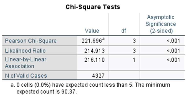
The chi-square test statistic is X2 = 221.7 on 3 df gives a p-value of P<0.001. The p value of the chi-square test is highly significant (p<0.001), suggesting that we can reject the null hypothesis that there is no difference in true fatal CVD prevalence across different age groups. While we can observe in the row percentages that fatal CVD prevalence is the highest at older ages, and lowest at younger ages, the chi-square test is a global test so it just tells us there is a difference somewhere in the table; it does not tell us which groups are different nor does it tell us about the nature of the association (e.g. if it is positive or negative).
Chi-square test for linear trend
In this example we are going to look for a linear trend between fatal CVD and age group.
The chi-square test for linear trend (also called the Cochran-Armitage test for linear trend) is used with case-control and cross-sectional data, and it estimates the ratio of the odds of failure (i.e. disease) for two categories of explanatory variables. It then tests whether this odds ratio is equal to 1.
SPSS does not run this exact test, which allows comparison of multiple groups. Instead you would use the Cochran-Mantel-Haenzel Test, which does the same thing, but will only run the trend test on two groups at a time. This means we firstly need to select the groups we want to compare. CVD death only contain two groups, so this is fine. For age group, we will just select the first and second groups to work on (groups 1 and 2), using the select cases function. You learnt how to do this in practical B3.5.
Select
Data >> Select Cases.
Then tick ‘If condition is satisfied’ click on the ‘If’ button and use If age_grp =< 2, then press OK. You will then see a strike though line appear on the row ID number of all rows containing data from participants in ages groups 3 and 4, indicating that these will not be included in the analysis.
This test does not require calculation of risk ratios, so it does not matter how the binary variables are coded in SPSS. In these examples we have used the default of No= 0 and Yes =1.
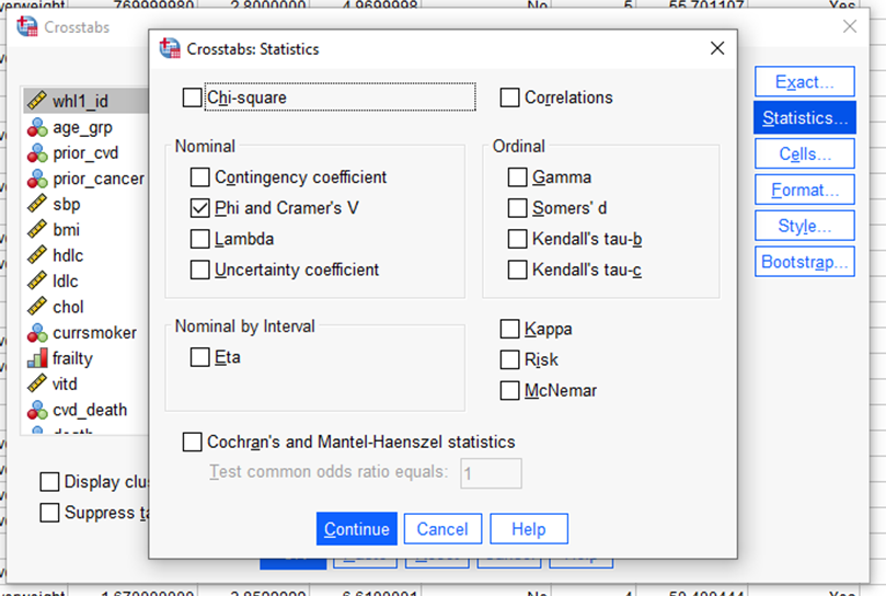
Now we use the ‘Crosstabs’ function as in the previous practical, but we tick ‘Cochran’s and Mantel-Haenszal statistics under the ‘Statistics’ tab. Leave the ‘test common odds ratio’ as the default value of one, this is the null hypothesis that we are testing against.

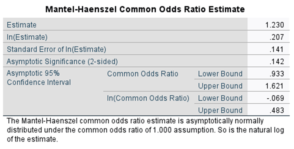
Again, SPSS gives lots of output tables, but the one we are interested in looks like the below.

The ‘estimate’ row is the odds ratio for fatal CVD death between the 60-70 years of age group and the 71-75 years of age group. The lower and upper bound are the of the common odds ratio are the 95% CO for the odds ratio, and the asymptotic significant is the p value for the relationship.
The other option we have for assessing trend in categorical variables in SPSS is Cramer’s V test. Again we can just tick the ‘Phi and Cramer’s V’ box in the ‘Crosstabs’ pop up to add this test into our analysis (Phi can be used instead of Cramer’s V for a 2 x 2 table, so SPSS groups these tests).
The value for Cramer’s V is a bit like a correlation coefficient for categorical data. A value of less than 0.1 is considered a very weak association, > 0.1 is a low association, > 0.3 is a moderate association, and > 0.5 is a strong association.
The Cramer’s V output would look like the below.

This indicates a statistically significant, low to moderate association between age group and fatal CVD.
Question C1.2b.i: Obtain the prevalence of prior diabetes in the different groups of BMI. What happens to diabetes prevalence as the BMI group increases?
Question C1.2b.ii: Perform tests of linear trend on these variables. What is the null hypothesis and what do the results of this test suggest?
Answer
The cross tabulation output will look like the below. The prevalence of diabetes changes from 8% (underweight) to 5.1% (normal weight) to 8.8% in the group with obesity.

For the Mantel-Haenszel analysis You will have three output tables for the three different comparisons of the side by side groupings.
Underweight vs Normal weight

Normal weight vs. Overweight
Overweight vs. Obese

The odds ratios suggest that the there is an increase in diabetes prevalence between the normal and overweight groups, and the overweight and obese groups, but the 95% CI crosses 0 for both of these comparisons, so the odds ratios do not significant differ from 1.
A Cramer’s V output for this association would look like the below.

Here it is indicating a significant correlation, or linear trend for increasing rates of diabetes as the BMI group increases (p=0.039) but the coefficient is very small (V=0.04), which indicates that this association is very weak.
C1.2 PRACTICAL: R
Performing the chi-square test for association
We want to look at the association of age group with fatal CVD. In order to obtain a chi-square test for association, we use the ‘chisq.test()’ command, and the output looks like this:
> chisq.test(df$age_grp, df$cvd_death, correct=FALSE)
Pearson’s Chi-squared test
data: df$age_grp and df$cvd_death
X-squared = 221.64, df = 3, p-value < 2.2e-16
- Question C1.2a: Is there an association between age group and fatal CVD? Just looking at a cross-tabulation table without doing any additional steps, are you able to tell which age groups are different from each other?
Answer
Answer C1.2a The chi-square test statistic is shown below the table and is X2 = 221.6 on 3 df (chi2(3)) which gives a p-value of Pr <2.2E-16.
The p value of the chi-square test is highly significant (p<0.001), suggesting that we can reject the null hypothesis that there is no difference in true fatal CVD prevalence across different age groups. While we can observe in the row percentages that fatal CVD prevalence is the highest at older ages, and lowest at younger ages, the chi-square test is a global test so it just tells us there is a difference somewhere in the table; it does not tell us which groups are different nor does it tell us about the nature of the association (e.g if it is positive or negative).
Performing the chi-square test for linear trend (Cochran-Armitage test)
The chi-square test for linear trend (also called the Cochran-Armitage test for linear trend) is obtained using the ‘prop.trend.test()’ command. The setup of this command is:
prop.trend.test(x, n)
where:
- x is the number of events per group, and
- n is the total sample size per group
The output should look like this:
> table(df$age_grp, df$cvd_death)
0 1
1 788 45
2 1574 201
3 852 214
4 407 185
> cvd_agegrp <- c(45, 201, 214, 185)
> table(df$age_grp)
1 2 3 4
833 1775 1066 592
> total_agegrp <- c(833, 1775, 1066, 592)
> prop.trend.test( x=cvd_agegrp, n=total_agegrp)
Chi-squared Test for Trend in Proportions
data: cvd_agegrp out of total_agegrp ,using scores: 1 2 3 4
X-squared = 216.47, df = 1, p-value < 2.2e-16
Here, ‘X-squared’ refers to the chi-square test for linear trend, which yields a highly significant p-value.
- Question C1.2b.i: Obtain the prevalence of prior diabetes in the different groups of BMI. What happens to diabetes prevalence as the BMI group increases?
- Question C1.2b.ii: Perform a chi-square test of linear trend. What is the null hypothesis and what do the results of this test suggest?
C1.2b Answers
Answer C1.2b.i
The prevalence of diabetes increases from 8% (underweight) to 5% (normal weight) to 8.8% in the group with obesity.
> df$bmi_grp4 <- factor(df$bmi_grp4, levels=c(1,2,3,4), labels=c(“Underweight”, “Normal”, “Overweight”, “Obese”)))
> prop.table(table(df$bmi_grp4, df$prior_t2dm),1)
0 1
Underweight 0.91836735 0.08163265
Normal 0.94974591 0.05025409
Overweight 0.93913043 0.06086957
Obese 0.91223404 0.08776596
Answer C1.2b.ii
> table(df$bmi_grp4, df$prior_t2dm)
0 1
Underweight 45 4
Normal 1682 89
Overweight 1944 126
Obese 343 33
> t2dm_bmig <- c(4, 89, 126, 33)
> table(df$bmi_grp4)
Underweight Normal Overweight Obese
49 1771 2070 376
> total_bmig <- c(49, 1771, 2070, 376)
> prop.trend.test(x = t2dm_bmig , n = total_bmig )
Chi-squared Test for Trend in Proportions
data: t2dm_bmig out of total_bmig ,
using scores: 1 2 3 4
X-squared = 5.7849, df = 1, p-value = 0.01616
The chi-square test for linear trend is obtained using the ‘prop.trend.test()’ command. The chi-square value (for 1 degree of freedom) is 5.8 and the p-value=0.02. There is evidence of a significant linear trend, and we can reject the null hypothesis that there is no association between diabetes status and BMI group.
Great