-
Course Information
Meet the Teaching Team -
Course Dataset 1
-
Course Dataset 2
-
MODULE A1: INTRODUCTION TO STATISTICS USING R, STATA, AND SPSSA1.1 What is Statistics?
-
A1.2.1a Introduction to Stata
-
A1.2.2b: Introduction to R
-
A1.2.2c: Introduction to SPSS
-
A1.3: Descriptive Statistics
-
A1.4: Estimates and Confidence Intervals
-
A1.5: Hypothesis Testing
-
A1.6: Transforming Variables
-
End of Module A11 Quiz
-
MODULE A2: POWER & SAMPLE SIZE CALCULATIONSA2.1 Key Concepts
-
A2.2 Power calculations for a difference in means
-
A2.3 Power Calculations for a difference in proportions
-
A2.4 Sample Size Calculation for RCTs
-
A2.5 Sample size calculations for cross-sectional studies (or surveys)
-
A2.6 Sample size calculations for case-control studies
-
End of Module A21 Quiz
-
MODULE B1: LINEAR REGRESSIONB1.1 Correlation and Scatterplots
-
B1.2 Differences Between Means (ANOVA 1)
-
B1.3 Univariable Linear Regression
-
B1.4 Multivariable Linear Regression
-
B1.5 Model Selection and F-Tests
-
B1.6 Regression Diagnostics
-
End of Module B11 Quiz
-
MODULE B2: MULTIPLE COMPARISONS & REPEATED MEASURESB2.1 ANOVA Revisited – Post-Hoc Testing
-
B2.2 Correcting For Multiple Comparisons
-
B2.3 Two-way ANOVA
-
B2.4 Repeated Measures and the Paired T-Test
-
B2.5 Repeated Measures ANOVA
-
End of Module B21 Quiz
-
MODULE B3: NON-PARAMETRIC MEASURESB3.1 The Parametric Assumptions
-
B3.2 Mann-Whitney U Test
-
B3.3 Kruskal-Wallis Test
-
B3.4 Wilcoxon Signed Rank Test
-
B3.5 Friedman Test
-
B3.6 Spearman’s Rank Order Correlation
-
End of Module B31 Quiz
-
MODULE C1: BINARY OUTCOME DATA & LOGISTIC REGRESSIONC1.1 Introduction to Prevalence, Risk, Odds and Rates
-
C1.2 The Chi-Square Test and the Test For Trend
-
C1.3 Univariable Logistic Regression
-
C1.4 Multivariable Logistic Regression
-
End of Module C11 Quiz
-
MODULE C2: SURVIVAL DATAC2.1 Introduction to Survival Data
-
C2.2 Kaplan-Meier Survival Function & the Log Rank Test
-
C2.3 Cox Proportional Hazards Regression
-
C2.4 Poisson Regression
-
End of Module C21 Quiz
-
A Note about the Fossa Certificate


Learning Outcomes
By the end of this section, students will be able to:
- Explain when and how to use post hoc testing
- Explain the concept of multiple comparisons and be able to correct for it in their analysis
- Explain when and how to use repeated measures statistics
- Apply extensions to the basic ANOVA test and interpret their results
You can download a copy of the slides here: B2.2a Correcting for Multiple Comparisons
B2.2a PRACTICAL: ALL
False Discovery Rate
To use this method, we must first assign a value for q. Whereas α is the proportion of false positive tests we are willing to accept across the whole sample typically 0.05 (5%), q is the proportion of false positives (false ‘discoveries’) that we are willing to accept within the significant results. In this example we will set q to 0.05 (5%) as well.
Here we are going to apply the Benjamini-Hochberg (BH) method to the data from the Fishers LSD test in the previous practical in section B2.1
Firstly, take the P values for each comparison of pairs and put them in ascending numerical order. Then assign a rank number in that order (smallest P value is rank 1, next smallest rank 2 and so on).
| Group A | Group B | P | Rank |
| Normal | Obese | <0.001 | 1 |
| Normal | Overweight | 0.001 | 2 |
| Underweight | Obese | 0.013 | 3 |
| Overweight | Obese | 0.056 | 4 |
| Underweight | Overweight | 0.060 | 5 |
| Underweight | Normal | 0.246 | 6 |
Calculate the BH critical value for each P value, using the formula q(i/m), where:
i = the individual p-value’s rank,
m = total number of tests,
q= the false discovery rate you have selected (0.05)
| Group A | Group B | P | Rank | BHcrit | Significant |
| Normal | Obese | <0.001 | 1 | 0.008 | Yes |
| Normal | Overweight | 0.001 | 2 | 0.016 | Yes |
| Underweight | Obese | 0.013 | 3 | 0.025 | Yes |
| Overweight | Obese | 0.056 | 4 | 0.033 | No |
| Underweight | Overweight | 0.060 | 5 | 0.042 | No |
| Underweight | Normal | 0.246 | 6 | 0.050 | No |
P values which are lower than our BH critical values are considered true ‘discoveries’. The first P value which is higher than the BH critical value and all significant P values below that (below in terms of the table, higher rank numbers) would be considered false ‘discoveries’. P values of ≥0.05 are not treated any differently to normal.
From this we can conclude that all three of our statistically significant differences from out pairwise comparisons are in true ‘discoveries’, and none of them should be discounted.
With small numbers of comparisons like this it is easy to use this method by hand, however where the FDR approach is most useful is when we are making very large numbers (hundreds) of comparisons.
—-
To compute this in R use the code
BH(u, alpha = 0.05)
where u is a vector containing all of the P values, and alpha is in fact your specified value for q
—-
To compute this is Stata you need to download the package smileplot which contains the programme multploc. This will allow you to perform the BH test. More details can be seen on this here- https://www.rogernewsonresources.org.uk/papers/multproc.pdf
—-
In SPSS there is a function to do this test within one of the extension bundles, but you can create a variable which contains all of your P values and then conduct a calculation for BH critical values using the ‘compute variable’ function (see A1.6) then make a visual assessment.
—-
There are also online FDR calculator you can use like this one https://tools.carbocation.com/FDR.
Try analysing the data from our example with at least one other method to check your results.
You can download a copy of the slides here: B2.2b Correcting for Multiple Comparisons
B2.2b PRACTICAL: R
In Practical B2.1, we ran the Fisher’s LSD test to compare systolic blood pressure (SBP) between each possible pairing of groups in the BMI group categorical variable. Now we know a little be more about post hoc tests and correcting for multiple comparisons, we are going to go back and conduct the Bonferroni post hoc and Tukey’s HSD post hoc on the same data.
Tukey’s test in R
The function is ‘TukeyHSD’ (which comes loaded in R already so you do not need to install any packages). You run this function after you fit the ANOVA as you did in B2.1:
> model1<- aov(sbp~bmi_fact, data=white.data)
> summary(model1)

[output omitted]

> TukeyHSD(model1, conf.level = .95)
  Tukey multiple comparisons of means
    95% family-wise confidence level

Fit: aov(formula = sbp ~ bmi_fact, data = white.data)

$bmi_fact
        diff        lwr       upr     p adj
2-1 2.909514 -3.5381290  9.357157 0.6523423
3-1 4.706123 -1.7291986 11.141444 0.2370134
4-1 6.579362 -0.1897670 13.348490 0.0603475
3-2 1.796609  0.3476829  3.245534 0.0079012
4-2 3.669847  1.1189404  6.220755 0.0012615
4-3 1.873239 -0.6463616  4.392839 0.2235822
Bonferroni test in R
To perform a Bonferroni correction, you run the post estimation function ‘pairwise.t.test(x, g, p.adjust.method =’bonferroni’)’. Here ‘x’ is your response variable, ‘g’ is the grouping variable, and for p.adjust.method you specify ‘bonferroni’.
The output is:
> model1<- aov(sbp~bmi_fact, data=white.data)
> summary(model1)

[output omitted]

pairwise.t.test(white.data$sbp, white.data$bmi_grp4, p.adjust.method ='bonferroni')

 Pairwise comparisons using t tests with pooled SD

data:  white.data$sbp and white.data$bmi_grp4

     1      2      3
2 1.0000 -      -
3 0.3615 0.0087 -
4 0.0752 0.0013 0.3366

P value adjustment method: bonferroni
Consider the different post hoc tests and the results for each comparison in them. Is one method producing higher or lower p values than the others? Do any previously significant findings become non-significant after correction for multiple comparisons?
Answer
The table below shows the outcome for each of the possible pairs, for each of the three different post hoc tests. These have been ordered from smallest to largest p value for ease of comparison.
| Group A | Group B | P value | ||
| Fisher’s LSD | Tukey’s HSD | Bonferroni | ||
| Normal | Obese | <0.001* | 0.001* | 0.001* |
| Normal | Overweight | 0.001* | 0.008* | 0.009* |
| Underweight | Obese | 0.013* | 0.060 | 0.075 |
| Overweight | Obese | 0.056 | 0.224 | 0.337 |
| Underweight | Overweight | 0.060 | 0.237 | 0.361 |
| Underweight | Normal | 0.246 | 0.652 | 1.000 |
*= P<0.05- Reject H0
You should notice that the p-vales are lowest for each comparison on the LSD test, and highest in the Bonferroni. Once we apply a correction for multiple comparisons in this way the significant difference in SBP between underweight and obese groups disappears and we fail to reject the null hypothesis for this pairing.
B2.2b PRACTICAL: Stata
In Practical B2.1, we ran the Fisher’s LSD test to compare systolic blood pressure (SBP) between each possible pairing of groups in the BMI group categorical variable. Now we know a little be more about post hoc tests and correcting for multiple comparisons, we are going to go back and conduct the Bonferroni post hoc and Tukey’s HSD post hoc on the same data.
The post-estimation command ‘pwcompare’ with the ‘mcompare(method)’ option specifies the method for computing p-values and confidence intervals that account for multiple comparisons.
In the Fisher’s LSD example we used ‘mcompare(noadjust)’, meaning there is no adjustment for multiple comparisons.
To run the same test with Bonferroni post hoc replace this with ‘mcompare(bonferroni)’.
To run the Tukey’s post hoc replace this with ‘mcompare(tukey)’
See the output here:
quietly: anova sbp bmi_grp4
pwcompare bmi_grp4, mcompare(bonferroni) effects
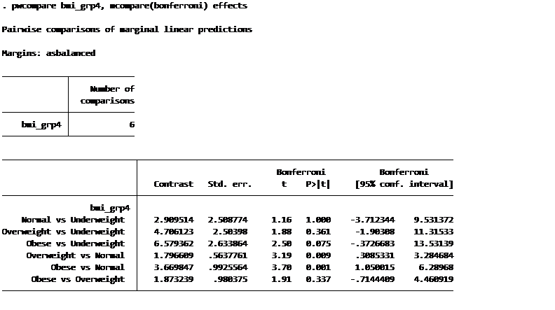
pwcompare bmi_grp4, mcompare(tukey) effects
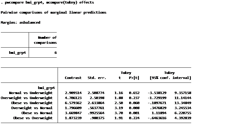
Consider the different post hoc tests and the results for each comparison in them. Is one method producing higher or lower p values than the others? Do any previously significant findings become non-significant after correction for multiple comparisons?
Answer
The table below shows the outcome for each of the possible pairs, for each of the three different post hoc tests. These have been ordered from smallest to largest p value for ease of comparison.
| Group A | Group B | P value | ||
| Fisher’s LSD | Tukey’s HSD | Bonferroni | ||
| Normal | Obese | <0.001* | 0.001* | 0.001* |
| Normal | Overweight | 0.001* | 0.008* | 0.009* |
| Underweight | Obese | 0.013* | 0.060 | 0.075 |
| Overweight | Obese | 0.056 | 0.224 | 0.337 |
| Underweight | Overweight | 0.060 | 0.237 | 0.361 |
| Underweight | Normal | 0.246 | 0.652 | 1.000 |
*= P<0.05- Reject H0
You should notice that the p-vales are lowest for each comparison on the LSD test, and highest in the Bonferroni. Once we apply a correction for multiple comparisons in this way the significant difference in SBP between underweight and obese groups disappears and we fail to reject the null hypothesis for this pairing.
B2.2b PRACTICAL: SPSS
In Practical B2.1, we ran the Fisher’s LSD test to compare systolic blood pressure (SBP) between each possible pairing of groups in the BMI group categorical variable. Now we know a little be more about post hoc tests and correcting for multiple comparisons, we are going to go back and conduct the Bonferroni post hoc and Tukey’s HSD post hoc on the same data.
Run the ANOVA in exactly the same way as before, but when you reach the screen where you tick the box next to your choice of post hoc tests, select ‘Bonferroni’ and ‘Tukey’.

Consider the different post hoc tests and the results for each comparison in them. Is one method producing higher or lower p values than the others? Do any previously significant findings become non-significant after correction for multiple comparisons?
Answer
The table below shows the outcome for each of the possible pairs, for each of the three different post hoc tests. These have been ordered from smallest to largest p value for ease of comparison.
| Group A | Group B | P value | ||
| Fisher’s LSD | Tukey’s HSD | Bonferroni | ||
| Normal | Obese | <0.001* | 0.001* | 0.001* |
| Normal | Overweight | 0.001* | 0.008* | 0.009* |
| Underweight | Obese | 0.013* | 0.060 | 0.075 |
| Overweight | Obese | 0.056 | 0.224 | 0.337 |
| Underweight | Overweight | 0.060 | 0.237 | 0.361 |
| Underweight | Normal | 0.246 | 0.652 | 1.000 |
*= P<0.05- Reject H0
You should notice that the p-vales are lowest for each comparison on the LSD test, and highest in the Bonferroni. Once we apply a correction for multiple comparisons in this way the significant difference in SBP between underweight and obese groups disappears and we fail to reject the null hypothesis for this pairing.
Running the code BH(u, alpha = 0.05) in R requires specified packages and libraries that were not given in the notes. The online FDR calculator provided was used instead
I did with the following script dear james
### Get the raw p-values from pairwise comparisons (for example with Tukey):
tukey_res <- TukeyHSD(model1, “bmi_fact”)
pvals <- tukey_res$bmi_fact[, “p adj”]
### Here pvals is a vector of p-values from all comparisons.
## Apply Benjamini–Hochberg adjustment:
pvals_fdr <- p.adjust(pvals, method = “BH”)
pvals_fdr
### This gives you the adjusted p-values (the equivalent of what BH(u, alpha=0.05) was meant to represent).