-
Course Information
Meet the Teaching Team -
Course Dataset 1
-
Course Dataset 2
-
MODULE A1: INTRODUCTION TO STATISTICS USING R, STATA, AND SPSSA1.1 What is Statistics?
-
A1.2.1a Introduction to Stata
-
A1.2.2b: Introduction to R
-
A1.2.2c: Introduction to SPSS
-
A1.3: Descriptive Statistics
-
A1.4: Estimates and Confidence Intervals
-
A1.5: Hypothesis Testing
-
A1.6: Transforming Variables
-
End of Module A11 Quiz
-
MODULE A2: POWER & SAMPLE SIZE CALCULATIONSA2.1 Key Concepts
-
A2.2 Power calculations for a difference in means
-
A2.3 Power Calculations for a difference in proportions
-
A2.4 Sample Size Calculation for RCTs
-
A2.5 Sample size calculations for cross-sectional studies (or surveys)
-
A2.6 Sample size calculations for case-control studies
-
End of Module A21 Quiz
-
MODULE B1: LINEAR REGRESSIONB1.1 Correlation and Scatterplots
-
B1.2 Differences Between Means (ANOVA 1)
-
B1.3 Univariable Linear Regression
-
B1.4 Multivariable Linear Regression
-
B1.5 Model Selection and F-Tests
-
B1.6 Regression Diagnostics
-
End of Module B11 Quiz
-
MODULE B2: MULTIPLE COMPARISONS & REPEATED MEASURESB2.1 ANOVA Revisited – Post-Hoc Testing
-
B2.2 Correcting For Multiple Comparisons
-
B2.3 Two-way ANOVA
-
B2.4 Repeated Measures and the Paired T-Test
-
B2.5 Repeated Measures ANOVA
-
End of Module B21 Quiz
-
MODULE B3: NON-PARAMETRIC MEASURESB3.1 The Parametric Assumptions
-
B3.2 Mann-Whitney U Test
-
B3.3 Kruskal-Wallis Test
-
B3.4 Wilcoxon Signed Rank Test
-
B3.5 Friedman Test
-
B3.6 Spearman’s Rank Order Correlation
-
End of Module B31 Quiz
-
MODULE C1: BINARY OUTCOME DATA & LOGISTIC REGRESSIONC1.1 Introduction to Prevalence, Risk, Odds and Rates
-
C1.2 The Chi-Square Test and the Test For Trend
-
C1.3 Univariable Logistic Regression
-
C1.4 Multivariable Logistic Regression
-
End of Module C11 Quiz
-
MODULE C2: SURVIVAL DATAC2.1 Introduction to Survival Data
-
C2.2 Kaplan-Meier Survival Function & the Log Rank Test
-
C2.3 Cox Proportional Hazards Regression
-
C2.4 Poisson Regression
-
End of Module C21 Quiz
-
A Note about the Fossa Certificate


Learning Outcomes
By the end of this section, students will be able to:
-
- Explore the data with correlations and scatterplots.
- Use an ANOVA to test for a difference in means across a categorical variable.
- Conduct univariable and multivariable linear regression
- Check the regression diagnostics of a linear model.
You can download a copy of the slides here: B1.3 Univariable Linear Regression
Video B1.3a – The Regression Line (7 minutes)
You can download a copy of the slides here: B1.3b Univariable Linear Regression
Video B1.3b – Linear Model with One Continuous Independent Variable (7 minutes)
B1.3a PRACTICAL: Stata
Linear regression with a continuous exposure
In section B1.1 we examined the association between two continuous variables (SBP and BMI [continuous]) using scatterplots and correlations. We can also assess the relationship between two continuous variables by using linear regression. In comparison with the regression using a categorical exposure, if we have a continuous variable we interpret the beta coefficient as the “average increase in [outcome] for a 1 unit change in [exposure]’.
The code for linear regression is:
regress outcome exposure [, options]
Try this for SBP and continuous BMI:
regress sbp bmi
Question 1.3a: What conclusions do you make about the relationship between SBP and BMI [continuous]?
Answer

For every 1 unit higher BMI, SBP on average increases 0.46 mmHg (95% CI: 0.30-0.62), and this association is statistically significant (p<0.001).
B1.3a PRACTICAL: SPSS
Linear regression with a continuous exposure
In section B1.1 we examined the association between two continuous variables (SBP and BMI [continuous]) using scatterplots and correlations. We can also assess the relationship between two continuous variables by using linear regression. In comparison with the regression using a categorical exposure, if we have a continuous variable we interpret the beta coefficient as the “average increase in [outcome] for a 1 unit change in [exposure]’.
Try this for SBP and continuous BMI.
Select
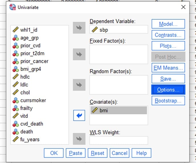
Analyze >> General Linear Model > Univariate
This time put the SBP into the Dependant Variable box and put continuous BMI into the Covariates box. As before, make sure ‘Parameter Estimates’ is selected in the Options tab.
What conclusions do you make about the relationship between SBP and BMI [continuous]?
Answer
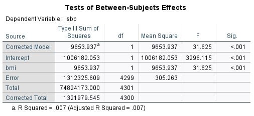

For every 1 unit higher BMI, SBP on average increases 0.46 mmHg (95% CI: 0.30-0.62), and this association is statistically significant (p<0.001)
B1.3a PRACTICAL: R
Linear regression with continuous exposure
In section B1.1 we examined the association between two continuous variables (SBP and BMI [continuous]) using scatterplots and correlations. We can also assess the relationship between two continuous variables by using linear regression. In comparison with the regression using a categorical exposure, if we have a continuous variable we interpret the beta coefficient as the “average increase in [outcome] for a 1 unit change in [exposure]’.
We can fit a simple linear regression model to the data using the lm() function as lm(formula, data)and the fitted model can be saved to an object for further analysis. For example my.fit <- lm(Y ~ X, data = my.data) performs a linear regression of Y (response variable) versus X (explanatory variable) by taking them from the dataset my.data. The result is stored on an object called my.fit.
Other different functional forms for the relationship can be specified via formula. The data argument is used to tell R where to look for the variables used in the formula.
When the model is saved in an object we can use the summary() function to extract information about the linear model (estimates of parameters, standard errors, residuals, etc). The function confint() can be used to compute confidence intervals of the estimates in the fitted model.
Let us now fit a linear regression model with SBP as our response variable, and continuous BMI as our explanatory variable.
> fit1 <- lm(sbp ~ bmi, data=white.data)
> summary(fit1)
Question 1.3a: Fit a linear model of SBP versus BMI (continuous) in the Whitehall data and interpret your findings.
Answer
> fit1 <- lm(sbp ~ bmi, data=white.data)
> summary(fit1)
Call:
lm(formula = sbp ~ bmi, data = white.data)
Residuals:
Min 1Q Median 3Q Max
-43.087 -12.169 -1.710 9.831 101.667
Coefficients:
Estimate Std. Error t value Pr(>|t|)
(Intercept) 119.15237 2.07540 57.412 < 2e-16 ***
bmi 0.45902 0.08162 5.624 1.99e-08 ***
—
Signif. codes: 0 ‘***’ 0.001 ‘**’ 0.01 ‘*’ 0.05 ‘.’ 0.1 ‘ ’ 1
Residual standard error: 17.47 on 4299 degrees of freedom
(26 observations deleted due to missingness)
Multiple R-squared: 0.007303, Adjusted R-squared: 0.007072
F-statistic: 31.62 on 1 and 4299 DF, p-value: 1.989e-08
> confint(fit1)
2.5 % 97.5 %
(Intercept) 115.083517 123.221220
bmi 0.298996 0.619046
For every 1 unit higher BMI, SBP on average increases 0.46 mmHg (95% CI: 0.30-0.62), and this association is statistically significant (p<0.001)
Video B1.3c – Linear Model with One Binary Exposure (13 minutes)
Video B1.3d – Linear Model with One Categorical Exposure (7 minutes)
B1.3b PRACTICAL: Stata
Linear regression with a categorical exposure
Besides ANOVA, another way to assess differences in the mean of a continuous outcomes variable across groups is to use a linear regression. We could run a linear regression to compare the mean difference in each BMI group compared to a reference category. The code for linear regression is:
regress outcome exposure [, options]
Substitute SBP for the outcome and ‘bmi_grp4’ for the exposure, and run a linear regression (we do not want to specify any special options). Remember that bmi_grp4 is a factor (or categorical) variable, so you need to indicate this to Stata by putting the prefix “i.” before bmi_grp4, so it becomes “i.bmi_grp4”.
Question 1.3b.i: Fit a linear model of SBP versus bmi_grp4 and interpret your findings.
B1.3b. Answers
regress sbp i.bmi_grp4

Compared to underweight participants, normal weight participants have a mean SBP that is on average 2.9 mmHg higher (95% CI: -2-7.8). This is not statistically significant (p=0.25). Compared to underweight participants, participants with obesity have an average SBP that is 6.6 mmHg higher (95% CI 1.4-11.7) and this is statistically significant (p=0.013). The ‘_cons’ in the output is the average SBP in the reference group. In this case, this indicates the mean SBP in the underweight group is 126.7 mmHg.
You can examine different comparisons across the BMI variable by changing the baseline category by specifying ‘ib3.bmi_grp4’ in the command line. This syntax tells Stata that we want the 3 level of the bmi_grp4 variable to be the baseline (rather than the default, which is level 1). We would then see all the other levels of bmi_grp4 compared to level 3. Try this for yourself and see.
B1.3b PRACTICAL: SPSS
Linear regression with a categorical exposure
Besides ANOVA, another way to assess differences in the mean of a continuous outcomes variable is to use a linear regression. We could run a linear regression to compare the mean difference in each BMI group compared to a reference category.
There is a linear regression function in SPSS, but we will use the general linear model function instead, as this gives us more flexibility (most of the time).
Select
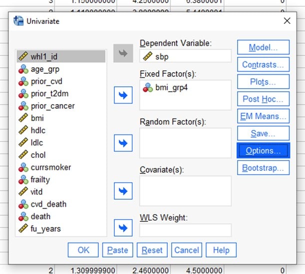
Analyze>> General Linear Model >> Univariate
Move SBP into the Dependent Variable box and the BMI groups variable(bmi_grp4) into the Fixed Factors box.
Then click on ‘Options’ on the right hand side and tick the box next to ‘Parameter Estimates’
Use this process to fit a linear model of SBP versus bmi_grp4 and interpret your findings. Write down the final form of the regression model. Interpret the coefficients of the model- what do they really mean?
Answer
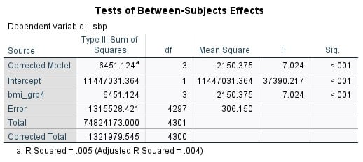

If you look at the top table, you will see that the F value and the significance value for the model are the same as for the ANOVA in the previous exercise. That is because these two methods are based on the same basic process.
The Parameter estimates table compares each of the BMI groups to the Obese group and explains how we can predict the SBP based on group.
Compared to underweight participants, participants with obesity have an average SBP that is 6.6 mmHg higher (95% CI 1.4-11.7) and this is statistically significant (p=0.013). In this case, this indicates the mean SBP in the underweight group is 126.7 mmHg. You can use the table to explain the relationships of the normal and overweight groups to the obese group in the same terms.
There are ways to compare all of the different groups to each other in SPSS. This is dealt with in Module B2.
In this scenario we end up with a simple predicative regression model of SBP= 133.2mmHg for the obese group (- 6.6 for underweight, – 3.7 for normal weight and -1.9 overweight). As there are no other variables in the model at this stage, the equation is just predicting based on the mean SBP of each group.
B1.3b PRACTICAL: R
Linear regression with categorical exposure
Instead of conducting multiple pairwise comparisons in an ANOVA, we could run a linear regression to compare the mean difference in each age group compared to a reference category.
First, we need to tell R to treat our exposure as a categorical variable:
white.data$bmi_fact<-factor(white.data$bmi_grp4)
We can use is.factor() to check that the new created variable is indeed a factor variable.
is.factor(white.data$bmi_fact)
## [1] TRUE
Then, we use table() to count the number of participants in each BMI category.
table(white.data$bmi_fact)
##
## 1 2 3 4
## 50 1793 2091 376
We can use aggregate() to compute summary statistics for SBP by BMI.
aggregate(white.data$sbp, list(white.data$bmi_fact), FUN=mean, na.rm=TRUE)
## Group.1 x
## 1 1 126.6600
## 2 2 129.5695
## 3 3 131.3661
## 4 4 133.2394
The results indicate that there are mean SBP increases across the four categories of BMI.
Now we fit a linear regression model called fit2 with SBP as our response and BMI groups as our explanatory variable.
fit2 <- lm(sbp ~ bmi_fact, data=white.data)
summary(fit2)
Call:
lm(formula = sbp ~ bmi_fact, data = white.data)
Residuals:
Min 1Q Median 3Q Max
-43.366 -12.239 -1.570 9.634 100.430
Coefficients:
Estimate Std. Error t value Pr(>|t|)
(Intercept) 126.660 2.474 51.187 <2e-16 ***
bmi_fact2 2.910 2.509 1.160 0.2462
bmi_fact3 4.706 2.504 1.879 0.0602 .
bmi_fact4 6.579 2.634 2.498 0.0125 *
If we want confidence intervals, we could then type:
confint(fit2, level=0.95)
By default R will use the lowest category of bmi_fact as the reference in a regression. But this category is the smallest and hence it is not a good reference category as all comparisons with it will have large confidence intervals. We can change the reference category using the ‘relevel’ function:
white.data<-within(white.data,bmi_fact<-relevel(bmi_fact,ref=2))
Then we fit the same linear regression again:
> fit2 <- lm(sbp ~ bmi_fact, data=white.data)
> summary(fit2)
> confint(fit2, level=0.95)
Question 1.3b: Using the new reference category of BMI group=2, what conclusions do you make about the relationship between SBP and BMI groups based on the regression output given by summary(fit2)?
Answer
Call:
lm(formula = sbp ~ bmi_fact, data = white.data)
Residuals:
Min 1Q Median 3Q Max
-43.366 -12.239 -1.570 9.634 100.430
Coefficients:
Estimate Std. Error t value Pr(>|t|)
(Intercept) 129.5695 0.4134 313.389 < 2e-16 ***
bmi_fact1 -2.9095 2.5088 -1.160 0.246221
bmi_fact3 1.7966 0.5638 3.187 0.001449 **
bmi_fact4 3.6698 0.9926 3.697 0.000221 ***
—
Signif. codes: 0 ‘***’ 0.001 ‘**’ 0.01 ‘*’ 0.05 ‘.’ 0.1 ‘ ’ 1
> confint(fit2, level=0.95)
2.5 % 97.5 %
(Intercept) 128.7589451 130.380083
bmi_fact1 -7.8280063 2.008978
bmi_fact3 0.6913165 2.901901
bmi_fact4 1.7239246 5.615770
Looking at the output above, the average level of SBP increases as BMI groups get higher. For a BMI group 4 (obese) compared to BMI group 2 (normal weight), the average SBP is 3.7 mmHg higher (95% CI: 1.7-5.6, p<0.001).